We follow the Megatron-LM / NeMo Megatron Bridge stack: names, grouping, and CLI flags line up with the training code and official parallelisms guide1,2. The tables below are a parameter-centric cheat sheet. For the ideas behind them—tensor parallelism3, pipeline parallelism and bubble-aware schedules2,4, sequence parallelism in the tensor-parallel group5, context-parallel long-sequence attention (including Ulysses-style all-to-all patterns)2,6, and expert-parallel MoE2,7—see Related Works.
In this section, we will summarize all parallelism-related parameters as well as their details.
We follow the categories of parallelism as defined in the Megatron Bridge1: Model Parallelism (TP, PP, EP), Activation Partitioning (SP, CP), and Data Parallelism (DP).
| Category | Strategies | What gets split |
|---|---|---|
| Data Parallelism | DP | Input data (batches) |
| Model Parallelism | TP, PP, EP | Model weights |
| Activation Partitioning | SP, CP | Intermediate activations (along sequence dim) |
| Parameter | Default | What it does |
|---|---|---|
--tensor-model-parallel-size |
1 |
Number of GPUs to split each weight matrix across (per layer) |
--tp-comm-overlap |
False |
Overlap TP all-gather / reduce-scatter with the matmul that produced or consumes them |
--tp-comm-overlap-cfg |
None |
Path to a YAML file with per-layer TP overlap settings |
--tp-comm-bootstrap-backend |
'nccl' |
Bootstrap backend used by TP-overlap ('nccl', 'mpi', 'gloo') |
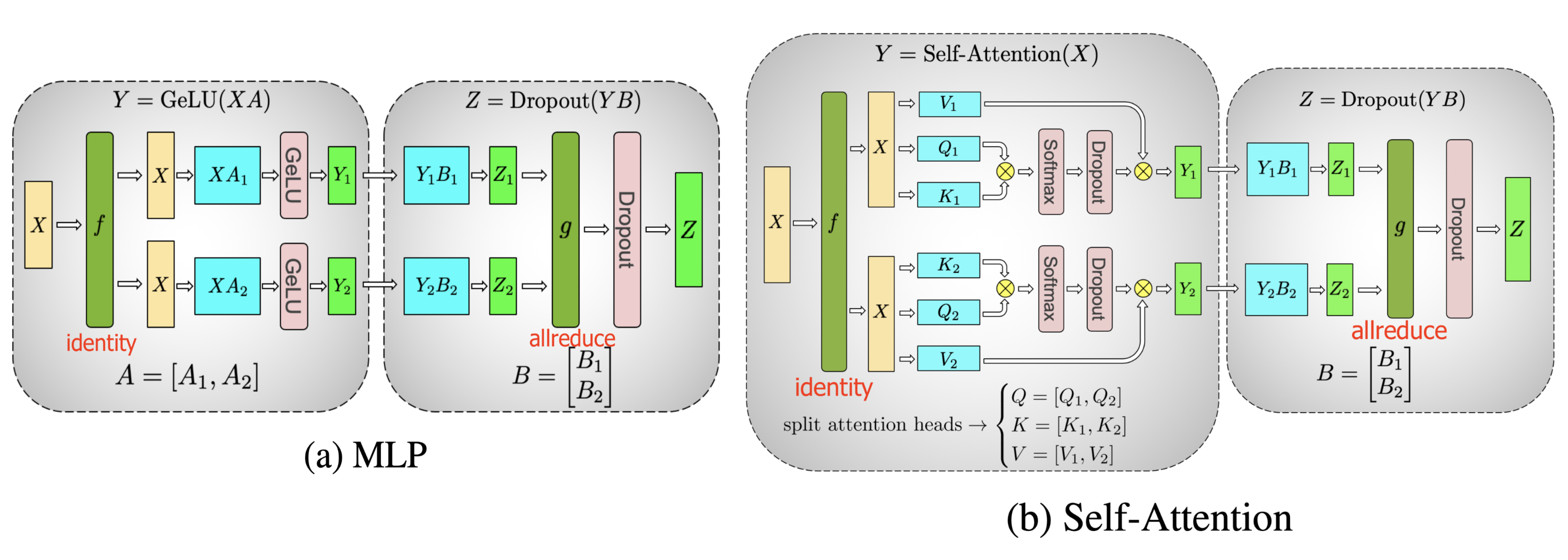
Forget about the Dropout here in the figure, we will check it over the SP section.
so let's start from a simple example of FFN (dense, no MoE), which is more easy to understand:
$$X \in \mathbb{R}^{S \times H}, \qquad W_{\mathrm{up}} \in \mathbb{R}^{H \times H_{\mathrm{ffn}}}, \qquad W_{\mathrm{down}} \in \mathbb{R}^{H_{\mathrm{ffn}} \times H}$$Without TP, it is:
$$Y = \phi(XW_{\mathrm{up}});\quad Z = YW_{\mathrm{down}};\quad Z = \phi(XW_{\mathrm{up}})W_{\mathrm{down}}$$With TP=4, we split along $H_{\mathrm{ffn}}$:
$$W_{\mathrm{up}} = \big[ W_{\mathrm{up}}^{(1)}, W_{\mathrm{up}}^{(2)}, W_{\mathrm{up}}^{(3)}, W_{\mathrm{up}}^{(4)} \big]$$ $$W_{\mathrm{down}} = \begin{bmatrix} W_{\mathrm{down}}^{(1)} \\ W_{\mathrm{down}}^{(2)} \\ W_{\mathrm{down}}^{(3)} \\ W_{\mathrm{down}}^{(4)} \end{bmatrix}$$where
$$W_{\mathrm{up}}^{(i)} \in \mathbb{R}^{H \times H_{\mathrm{ffn}}/4}, \qquad W_{\mathrm{down}}^{(i)} \in \mathbb{R}^{H_{\mathrm{ffn}}/4 \times H}$$So on GPU i:
$$Y_i = \phi\!\left(XW_{\mathrm{up}}^{(i)}\right); Z_i = Y_i W_{\mathrm{down}}^{(i)}$$Then the final output is $Z = \sum_{i=1}^{4} Z_i$. The derivation is as follows:
Equivalently, $Y = [Y_1, Y_2, Y_3, Y_4]$, and
$$W_{\mathrm{down}} = \begin{bmatrix} W_{\mathrm{down}}^{(1)} \\ W_{\mathrm{down}}^{(2)} \\ W_{\mathrm{down}}^{(3)} \\ W_{\mathrm{down}}^{(4)} \end{bmatrix}$$so
$$\begin{aligned} Z &= YW_{\mathrm{down}} \\ &= [Y_1, Y_2, Y_3, Y_4] \begin{bmatrix} W_{\mathrm{down}}^{(1)} \\ W_{\mathrm{down}}^{(2)} \\ W_{\mathrm{down}}^{(3)} \\ W_{\mathrm{down}}^{(4)} \end{bmatrix} \\ &= Y_1W_{\mathrm{down}}^{(1)} + Y_2W_{\mathrm{down}}^{(2)} + Y_3W_{\mathrm{down}}^{(3)} + Y_4W_{\mathrm{down}}^{(4)} \\ &= Z_1 + Z_2 + Z_3 + Z_4 \end{aligned}$$then let's move to Attention, which is a little bit more complex. But the basic idea is still the same.
Let's consider the vanilla Self-Attention:
$$\begin{aligned} X &\in \mathbb{R}^{S \times H}, \qquad W_Q, W_K, W_V, W_O \in \mathbb{R}^{H \times H} \end{aligned}$$ $$Q = XW_Q,\qquad K = XW_K,\qquad V = XW_V$$For head h, where $d_{\text{head}} = H / N_h$,
$$Q_h, K_h, V_h \in \mathbb{R}^{S \times d_{\text{head}}}$$ $$\mathrm{Attn}_h = \mathrm{softmax}\!\left(\frac{Q_h K_h^\top}{\sqrt{d_{\text{head}}}}\right)V_h \in \mathbb{R}^{S \times d_{\text{head}}}$$Concatenate all heads:
$$A = \mathrm{Concat}\!\left(\mathrm{Attn}_1, \dots, \mathrm{Attn}_{N_h}\right) \in \mathbb{R}^{S \times H}$$Output projection:
$$O = A W_O \in \mathbb{R}^{S \times H}$$With tensor parallelism
We split heads across GPUs, since heads are decoupled in the attention mechanism. (say, for context, you get this qi,kj problem)
Let TP degree be p=4. Split heads across GPUs, so each GPU holds $N_h/p$ heads.
$$\begin{aligned} W_Q &= [W_{Q,1}\; W_{Q,2}\; \cdots \; W_{Q,p}], \qquad \\ W_K &= [W_{K,1}\; W_{K,2}\; \cdots \; W_{K,p}], \qquad \\ W_V &= [W_{V,1}\; W_{V,2}\; \cdots \; W_{V,p}] \end{aligned}$$where
$$W_{Q,i}, W_{K,i}, W_{V,i} \in \mathbb{R}^{H \times H/p}$$and split $W_O$ row-wise:
$$W_O = \begin{bmatrix} W_{O,1} \\ W_{O,2} \\ \vdots \\ W_{O,p} \end{bmatrix}, \qquad W_{O,i} \in \mathbb{R}^{H/p \times H}$$On GPU i:
$$\begin{aligned} Q_i &= X W_{Q,i}, \qquad \\ K_i &= X W_{K,i}, \qquad \\ V_i &= X W_{V,i} \end{aligned}$$with
$$Q_i, K_i, V_i \in \mathbb{R}^{S \times H/p}$$GPU i computes attention only for its own head subset:
$$A_i = \mathrm{Attention}(Q_i, K_i, V_i) \in \mathbb{R}^{S \times H/p}$$Then local output projection:
$$O_i = A_i W_{O,i} \in \mathbb{R}^{S \times H}$$Each O_i is a partial sum. Final output:
$$O = \sum_{i=1}^{p} O_i$$equivalently,
$$O = \mathrm{AllReduce}\big(O_1, O_2, \dots, O_p\big)$$Why this works
Since
$$A = [A_1 \; A_2 \; \cdots \; A_p]$$and
$$W_O = \begin{bmatrix} W_{O,1} \\ W_{O,2} \\ \vdots \\ W_{O,p} \end{bmatrix},$$we have
$$\begin{aligned} O &= A W_O \\ &= [A_1 \; A_2 \; \cdots \; A_p] \begin{bmatrix} W_{O,1} \\ W_{O,2} \\ \vdots \\ W_{O,p} \end{bmatrix} \\ &= \sum_{i=1}^{p} A_i W_{O,i} \\ &= \sum_{i=1}^{p} O_i \end{aligned}$$Takeaway: matrix multiply with a block-partitioned inner dimension is a sum of independent sub-products. That's why AllReduce (sum) gives the exact answer.
1. X (full) × W_first_i (sharded)  →  intermediate_i (sharded) | no comm
2. compute on intermediate_i independently                     | no comm
3. intermediate_i × W_last_i (sharded)  →  partial_sum_i       | no comm
4. AllReduce(partial_sums)  →  correct output                  | 1 AllReduce
Takeaway: VPP is the best you can do in upstream Megatron. The research frontier has moved on to zero-bubble variants, and DeepSeek uses DualPipe in production — but adopting either requires patching a fork.
PP cuts the model's layers into sequential chunks and places each chunk on a different GPU. A forward pass becomes a relay — GPU 0 runs its layers, hands the activation to GPU 1, and so on. Backward flows in reverse.
The communication between adjacent stages is small (one activation tensor per hand-off), and only between neighbors — which is why PP is the natural choice for crossing slow inter-node links (InfiniBand) where TP's all-reduce bandwidth would be too expensive.
Consider a single micro-batch flowing through a 4-stage pipeline:
PP=4, M=1; F/B each take one slot; communication time omitted.
.. = idle

Time:   00 01 02 03 04 05 06 07
GPU 0:  F0 .. .. .. .. .. .. B0
GPU 1:  .. F0 .. .. .. .. B0 ..
GPU 2:  .. .. F0 .. .. B0 .. ..
GPU 3:  .. .. .. F0 B0 .. .. ..
Only one GPU works at a time — three GPUs sit idle at every step. This wasted idle time is the pipeline bubble. The fix: run many micro-batches in flight so that different stages process different micro-batches simultaneously.
How the bubble is filled depends on the schedule — the order in which forward (F) and backward (B) passes are dispatched. Every schedule is a different answer to the same packing problem: how to arrange F and B blocks on a PP×time grid to minimize empty cells.
The simplest multi-microbatch schedule4. Split the global batch into $M$ micro-batches. Run all forwards first, then all backwards:
PP=4, M=4; F/B each take one slot; communication time omitted.
.. = idle

Time:   00 01 02 03 04 05 06 07 08 09 10 11 12 13
GPU 0:  F0 F1 F2 F3 .. .. .. .. .. .. B3 B2 B1 B0
GPU 1:  .. F0 F1 F2 F3 .. .. .. .. B3 B2 B1 B0 ..
GPU 2:  .. .. F0 F1 F2 F3 .. .. B3 B2 B1 B0 .. ..
GPU 3:  .. .. .. F0 F1 F2 F3 B3 B2 B1 B0 .. .. ..
Two problems:
- Bubble: GPUs idle during warmup and cooldown. The exact bubble fraction is
which is approximately $(PP - 1) / M$ when $M \gg PP$. 2. Memory: every GPU must hold all $M$ micro-batches' activations until backward consumes them — peak activation memory blows up with $M$.
GPipe is the historical baseline. Nobody uses it today; it's here because every later schedule defines itself against it.
This is Megatron's
forward_backward_pipelining_without_interleaving.
The key insight: as soon as a backward becomes possible, do it immediately. After warmup, the pipeline enters a steady region where the last stage alternates forward and backward first, and earlier stages join that rhythm as gradients propagate back. This frees activation memory as soon as backward consumes it.
once a backward job becomes available, do it early, instead of piling up more and more forwards.
PP=4, M=7; F/B each take one slot; communication time omitted.
.. = idle

Time:   00 01 02 03 04 05 06 07 08 09 10 11 12 13 14 15 16 17 18 19
GPU 0:  F0 F1 F2 F3 .. .. .. B0 F4 B1 F5 B2 F6 B3 .. B4 .. B5 .. B6
GPU 1:  .. F0 F1 F2 .. .. B0 F3 B1 F4 B2 F5 B3 F6 B4 .. B5 .. B6 ..
GPU 2:  .. .. F0 F1 .. B0 F2 B1 F3 B2 F4 B3 F5 B4 F6 B5 .. B6 .. ..
GPU 3:  .. .. .. F0 B0 F1 B1 F2 B2 F3 B3 F4 B4 F5 B5 F6 B6 .. .. ..
The bubble fraction is still the same as GPipe:
$$\frac{PP - 1}{M + PP - 1}$$with the same large-$M$ approximation $(PP - 1) / M$. But the memory story is completely different: at any moment, GPU 0 holds activations for at most $PP$ micro-batches (not all $M$). That's a huge win when $M \gg PP$.
This is what 1F1B literally means: one forward, one backward, alternating in the steady state. It is Megatron's default PP schedule.
This is Megatron's
forward_backward_pipelining_with_interleaving, enabled by--virtual-pipeline-model-parallel-size.
The clever idea: make each pipeline stage shorter, so the bubble shrinks proportionally.
How? Each GPU holds multiple non-contiguous chunks of the model:
PP=4, VPP=2, 32 layers:
  GPU 0: chunks {0, 4} -> layers [0-3]   AND [16-19]
  GPU 1: chunks {1, 5} -> layers [4-7]   AND [20-23]
  GPU 2: chunks {2, 6} -> layers [8-11]  AND [24-27]
  GPU 3: chunks {3, 7} -> layers [12-15] AND [28-31]
A micro-batch's forward pass now traverses the GPUs VPP times instead of once:
cN = model chunk N; arrows show forward order

GPU0/c0 -> GPU1/c1 -> GPU2/c2 -> GPU3/c3
                                    |
                                    v
GPU3/c7 <- GPU2/c6 <- GPU1/c5 <- GPU0/c4
Each chunk is smaller (4 layers instead of 8), so the warmup time shrinks proportionally. In the simple equal-size-chunk model, the exact bubble fraction becomes:
$$\text{Bubble fraction with VPP} = \frac{PP - 1}{M \times VPP + PP - 1}$$For large $M$, this is approximately
$$\frac{PP - 1}{M \times VPP}$$so with $VPP=4$, the bubble approaches a $4\times$ reduction. The cost: more P2P communication, because each forward now does $VPP$ times more hand-offs between stages. Worth it on fast intra-node fabric; often worth it on InfiniBand too if $M$ is small.
Not in upstream Megatron. Reference implementation: sail-sg/zero-bubble-pipeline-parallelism. Also implemented in PyTorch's
torch.distributed.pipeliningasScheduleInterleavedZeroBubbleandScheduleZBVZeroBubble.
Zero Bubble (ZB)* is the first synchronous pipeline schedule to drive the bubble fraction to approximately zero. The trick is a finer decomposition of the backward pass.
The key insight: backward isn't atomic. Standard 1F1B treats B as one indivisible block. But the backward of a layer actually computes two distinct things:
- $B_{\text{input}}$ (call it
B): gradient with respect to the input activations. The previous stage needs this to start its own backward — so it's on the critical path of the pipeline. - $B_{\text{weight}}$ (call it
W): gradient with respect to the weights of this layer. Nothing downstream depends on this — it just gets accumulated into the optimizer's gradient buffer. SoWcan be deferred to any time before the optimizer step.
Once you split B into B + W, the scheduling problem changes shape. The pipeline still needs to honor F → B ordering across stages (the critical path), but W can be dropped into an available gap on its assigned GPU. The bubbles in 1F1B are exactly such gaps — and W can be sized to fill them.
Standard 1F1B:
  [B_input + B_weight] -> send dInput to the previous stage

Zero Bubble:
  [B_input]            -> send dInput to the previous stage
  [B_weight]           -> ready before the optimizer step
       ^
       can run later in a free slot on the same GPU

Dependencies only; horizontal positions are not timestamps.
Variants in the paper:
| Schedule | Memory | Bubble | Approach |
|---|---|---|---|
| ZB-H1 | $\sim$1F1B | small | Handcrafted, same memory as 1F1B |
| ZB-H2 | high | $\approx 0$ | Handcrafted, accepts higher memory for zero bubble |
| ZB-1P | $\sim$1F1B | small | Auto-searched (heuristic / integer linear programming), memory-matched to 1F1B |
| ZB-2P | high | <1% in most profiled settings | Auto-searched, the throughput champion (up to 31% faster than 1F1B) |
| ZB-V | $\sim$1F1B | small | V-shaped chunk dependency, comparable throughput to ZB-2P* |
(The "1/3 of 1F1B" figure sometimes quoted for ZB-V belongs to V-Min, a later memory-optimized schedule that gives up the zero bubble†.)
The reference implementation exposes a single knob: --zero-bubble-max-pending-backward. Setting it to 1 × PP gives you ZB-1P; 2 × PP gives you ZB-2P. ZB-V uses a separate flag (--zero-bubble-v-schedule) because its dependency structure is different.
One subtle requirement for true zero bubble: the optimizer step normally synchronizes across pipeline stages (so all stages step at the same boundary). The paper introduces a technique to bypass this synchronization, otherwise the optimizer-step barrier itself becomes a residual bubble.
When ZB beats 1F1B: essentially always (when the implementation is available). The original paper reports up to 23% over 1F1B under a similar memory limit, and up to 31% when the memory limit is relaxed*. ZB-V shows comparable throughput to the paper's ZB-2P* runs (half-sized micro-batches), with roughly 1F1B's activation-memory budget.
Not in upstream Megatron. Reference: deepseek-ai/DualPipe. Used in production for DeepSeek-V3/R1 training.
DualPipe‡ is DeepSeek's pipeline schedule for V3, designed specifically for MoE training where cross-node expert all-to-all has a ~1:1 compute-to-communication ratio — i.e., the all-to-all is so expensive it nearly equals the compute. Standard pipelining (even ZB) leaves this all-to-all exposed because there's no compute on the same micro-batch happening at the same time to hide behind. DualPipe creates that compute by running two micro-batch streams in opposite directions through the pipeline.
The bidirectional idea:
Same physical GPU order in every row:

Standard 1F1B:
  Forward:   GPU 0 -> GPU 1 -> GPU 2 -> GPU 3
  Backward:  GPU 0 <- GPU 1 <- GPU 2 <- GPU 3

DualPipe, forward directions:
  Stream A:  GPU 0 -> GPU 1 -> GPU 2 -> GPU 3
  Stream B:  GPU 0 <- GPU 1 <- GPU 2 <- GPU 3
  Each stream's backward runs opposite to its forward.

A possible overlap on GPU i (schematic, not to scale):
  A forward:  [EP dispatch        ]
  B backward: [independent compute]
The two streams' micro-batches don't share data. So on GPU 2 at time T:
- Stream A's forward might be running its all-to-all dispatch, while
- Stream B's backward is running its MLP compute, on a different stream
The two run in parallel — the all-to-all is hidden behind the unrelated MLP compute.
Fine-grained chunk decomposition. DualPipe takes ZB's idea further: every chunk is split into 4 components so that the scheduler can interleave them precisely:
| Component | What it is |
|---|---|
| Attention | The attention block compute |
| All-to-all dispatch | EP all-to-all that sends tokens to expert GPUs |
| MLP | Expert FFN compute (after dispatch) |
| All-to-all combine | EP all-to-all that returns expert outputs |
For backward chunks, both attention and MLP are further split into $B_{\text{input}}$ and $B_{\text{weight}}$ (the same trick as ZB). Plus a 5th component, the PP send/recv between stages.
Why the 4-way split matters: the scheduler can pair specific components from Stream A with independent components from Stream B. For example, Stream A's all-to-all dispatch overlaps with Stream B's attention compute — but communication kernels also use SMs, so overlap requires managing SM allocation and interference‡.
The cost. In the V3 report's comparison, DualPipe doubles per-device parameter memory (each device carries two chunks' weights), while peak activation memory is PP+1 micro-batches versus PP — not doubled activations‡. DeepSeek-V3 absorbs this cost because the alternative — leaving the cross-node all-to-all exposed — wastes far more wall-clock.
When DualPipe makes sense:
- MoE training where EP all-to-all dominates (DeepSeek-V3's exact situation)
- Cross-node PP where comm-heavy chunks need cover
- Memory headroom available for two in-flight streams
For dense models or smaller MoE, ZB is usually a better trade-off — same near-zero bubble without DualPipe's doubled parameter storage.
- *
Qi et al., "Zero Bubble Pipeline Parallelism," ICLR 2024. https://arxiv.org/abs/2401.10241v1. Schedule variants and flags: https://github.com/sail-sg/zero-bubble-pipeline-parallelism. ↩
- †
"Pipeline Parallelism with Controllable Memory," Table 1 distinguishes V-ZB, V-Half, and V-Min under the paper's balanced-stage model. https://arxiv.org/html/2405.15362v1. ↩
- ‡
DeepSeek-AI, "DeepSeek-V3 Technical Report," §2.1.2 (router), §3.2.1 and Table 2 (DualPipe), §3.2.2 and §3.5.1 (communication kernels and SM usage), §4.2 (model configuration). https://arxiv.org/html/2412.19437v2. Scheduler implementation: https://github.com/deepseek-ai/DualPipe. ↩
| Algorithm | Bubble fraction | Activation memory | Available in |
|---|---|---|---|
| GPipe | $(PP-1)/(M+PP-1)$ | All $M$ activations | Historical baseline |
| 1F1B | $(PP-1)/(M+PP-1)$ | $\leq PP$ activations | Megatron upstream |
| Interleaved 1F1B (VPP) | $(PP-1)/(M \cdot VPP + PP - 1)$ | Depends on VPP and warmup schedule§ | Megatron upstream |
| Zero Bubble (ZB-1P) | small | $\leq PP$ activations | sail-sg, PyTorch pipelining |
| Zero Bubble (ZB-2P) | $<1\%$ in most profiled settings* | $\sim 2 \times$ ZB-1P | sail-sg, PyTorch pipelining |
| Zero Bubble (ZB-V) | small | $\sim 1\times$ ZB-1P | sail-sg, PyTorch pipelining |
| DualPipe | $\approx 0$ | $2\times$ params, $(PP{+}1)/PP$ activations (V3 comparison) | DeepSeek's training code |
The exact fractions assume balanced stages (and for VPP, balanced virtual chunks). For $M \gg PP$, the first two reduce to the familiar approximation $(PP-1)/M$, and the interleaved schedule reduces to approximately $(PP-1)/(M \cdot VPP)$. The ZB-2P percentages are schedule calculations using profiled operation times, not guaranteed runtime bubble fractions*.
Takeaway: VPP is the best you can do in upstream Megatron. For Zero Bubble, drop into the sail-sg fork or use PyTorch's
torch.distributed.pipelining. For DualPipe, the DeepSeek-V3 training code is the reference. Neither is in upstream Megatron-LM as of this writing.
In an MoE (Mixture-of-Experts) model, each transformer block contains a router that sends tokens to a subset of many parallel FFN "experts." The whole point of MoE is to scale total parameters without scaling per-token compute — each token only activates its top-k experts. But those expert weights still live in memory. At scale this becomes the dominant cost: DeepSeek-V3, for example, has 256 routed experts per MoE layer, each a SwiGLU FFN with intermediate dim 2,048 on a hidden dim of 7,168 — about 44M params (~88 MB in bf16) per expert. One MoE layer's experts alone take ~22 GB; across all 58 MoE layers, total expert params exceed 1 TB. No single GPU can hold that. EP distributes experts across GPUs: with EP=8, each GPU holds 256/8 = 32 experts per layer, and tokens are routed to the right GPU via all-to-all communication.
| Parameter | Default | What it does |
|---|---|---|
--expert-model-parallel-size |
1 |
Number of GPUs to distribute MoE experts across |
--expert-tensor-parallel-size |
None |
TP within each expert; defaults to --tensor-model-parallel-size if not set |
--moe-token-dispatcher-type |
'allgather' |
Token routing mode: 'allgather', 'alltoall', or 'flex'. Use 'alltoall' (or 'flex') when applying expert parallelism |
--overlap-moe-expert-parallel-comm |
False |
Overlap the EP all-to-all communication with compute in 1F1B |
The big picture:
In a standard transformer block:
x -> Attention -> AddNorm -> FFN -> AddNorm -> next block
In an MoE block, the FFN is replaced by an MoE layer:
x -> Attention -> AddNorm -> MoE -> AddNorm -> next block
That's the only change. Attention stays the same.
token x ------> Router ------> top-k IDs + weights
      |
      | dispatch x using the selected IDs
      +---------------+---------------+
      |               |               |
      v               v               v
  Expert_3        Expert_17       Expert_42
    (FFN)           (FFN)           (FFN)
      |               |               |
      +---------------+---------------+
                      |
                      v
      weighted sum using router weights
                      |
                      v
                   output y
Router (a.k.a. gate)
- A tiny linear layer:
[hidden_dim -> num_experts] - Output: a logit per expert per token
- Apply softmax -> routing probabilities (DeepSeek-V3 uses sigmoid instead‡)
- Pick top-k experts per token (typically
k=2tok=8) - Renormalize the top-k probabilities so they sum to 1
Experts
-
Each expert is a full FFN, typically SwiGLU:
expert(x) = down_proj(silu(gate_proj(x)) * up_proj(x)) -
All experts have identical architecture but different weights
-
Number of experts: 8 (Mixtral), 64 (older small MoE), 256 (DeepSeek-V3), or more
-
Each expert is trained as a specialist over time, with no explicit specialization signal
Combine
-
Run
xthrough each of its top-k experts -
Weighted sum using the renormalized top-k router scores:
y = Σ_{e ∈ top_k} score_e * expert_e(x)
Per token, you have N experts in the model, but each token only touches k of them, where k << N.
- Total params scale with
N(number of experts) - Active params per token scale with
k - Compute per token =
k x (one expert), independent ofN
This is how MoE gets "more capacity at fixed compute." DeepSeek-V3 is 671B total parameters, but only 37B are active per token.
Without intervention, the router collapses: it learns to send most tokens to a few favorite experts, leaving others starved. Two standard fixes:
Auxiliary loss (most common): add a term to the training loss that penalizes uneven expert usage:
L_aux = N * Σ_e (frac_tokens_to_e * frac_router_prob_to_e)
This pushes the router toward uniform expert utilization.
Expert capacity / token dropping (older approach):
- Cap how many token-expert assignments each expert can process per batch (
ceil(capacity_factor x tokens x top_k / num_experts)) - If an expert is full, drop that token-expert assignment (other selected experts can still contribute)
- DeepSeek-V3 doesn't drop tokens; it uses other balancing tricks
Some MoE designs add shared experts: experts that every token always passes through, in addition to the routed top-k:
y = shared_expert(x) + Σ_{e ∈ top_k} score_e * routed_expert_e(x)
DeepSeek-V3 has 1 shared expert plus top-8 of 256 routed experts. The shared expert captures common features all tokens need, like grammar and basic syntax, which lets routed experts specialize more.
- Some models put MoE in every transformer block, such as Mixtral
- DeepSeek-V3 keeps the first 3 layers dense FFN, then uses MoE for layers 4-61 for stability
- Some research alternates MoE and dense layers
| Quantity | Value |
|---|---|
| Hidden dim | 7,168 |
| Routed experts per MoE layer | 256 |
| Shared experts per MoE layer | 1 |
| Top-k | 8 |
| Expert FFN intermediate (SwiGLU) | 2,048 |
| Per expert params | ~44M |
| Per MoE layer expert params | ~22.5 GB (bf16) |
| Total layers | 61 |
| Dense layers | 3 (first 3) |
| MoE layers | 58 |
| Total params | 671B |
| Active params per token | 37B |
MoE is "FFN sharded by function." Instead of one big FFN that processes every token, you have N small FFNs (experts) and a router that picks k of them per token. Compute per token stays fixed at k experts, but total model capacity scales with N. The router is trained jointly, often with an auxiliary loss to balance load. EP distributes those N experts across GPUs; without EP, every GPU would need to hold all experts and would run out of memory at scale.
Why
expert_tensor_parallel_size=1is the common choice
Dense TP makes sense because dense layers have large weight matrices. Consider a model with hidden_dim=7168:
Dense attention O-proj (TP=4):
[7168 × 7168] weight split into 4 chunks of [7168 × 1792]
Each chunk: 12.8M params — plenty of compute to justify the all-reduce.
Now consider the same TP applied to MoE experts. At DeepSeek-V3 scale (256 experts, each 7168 × 2048 SwiGLU), a single expert's up-proj is [7168 × 2048]. Split across expert_TP=4:
Each GPU's slice: [7168 × 512] — 3.7M params per projection, or about 11M for a full expert split (gate + up + down). The communication pattern changes too:
expert_TP=1:
Token → all-to-all dispatch → GPU runs the whole expert → all-to-all combine
Forward activation communication: 2 all-to-alls per MoE layer
expert_TP=4:
Token → all-to-all dispatch → AllGather tokens across the 4 expert-TP ranks → each rank computes its expert shard
→ ReduceScatter → all-to-all combine
Forward activation communication: 2 all-to-alls + one TP AllGather/ReduceScatter pair per MoE layer
These TP collectives run once per MoE layer on the batched dispatched tokens (steps 4 and 5 of the dispatcher walkthrough below) — not as one all-reduce per active expert¶.
The trade-off: expert_TP=1 means each expert must fit on one GPU, which is usually fine (a single DeepSeek-V3 expert is ~88 MB in bf16) — but a rank then holds all its local experts, plus their gradients and optimizer state. expert_TP>1 trades that aggregate memory for the extra collectives; it is not reserved for the case where a single expert doesn't fit.
So expert_TP=1 means: keep each expert whole on one GPU, and only use all-to-all to route tokens. That gives much less communication, while keeping enough compute per expert on each GPU to stay efficient.
- ¶
Megatron Core
core_v0.19.2, commit4b4acac9a1d28ea6829c8d4f566d75698a21249d: the MoE token dispatcher implements expert-TP as a batched AllGather/ReduceScatter around expert compute, not a per-expert all-reduce. ↩
How tokens get routed to the right experts when EP > 1. There are three modes:
allgather (the default, but only sensible without EP)
Wasteful when EP > 1 because every rank holds all tokens but only computes on a subset. Fine when EP = 1.
alltoall (the right choice for EP > 1)
The actual workflow is more involved than "just 2 all-to-alls." The full 7-step process from the code:
Preprocess— count tokens per destination and build the permutation indexPermute— reorder tokens contiguously by destination GPUA2A dispatch— NCCLall-to-all-von the EP group (every rank sends and receives variable-size chunks)Dispatch postprocess—AG(TP)ifexpert_TP > 1, then sort if there are multiple local expertsCombine preprocess— restore chunk order if there are multiple local experts, thenRS(TP)ifexpert_TP > 1A2A combine— NCCLall-to-all-von the EP group, with splits swappedUnpermute— reorder tokens back to original positions
Steps 4 and 5 include the TP AllGather and ReduceScatter that come into play only when expert_TP > 1. With expert_TP = 1 (the recommended config), those TP collectives are no-ops, but local-expert sorting can still be needed¶.
So: two EP activation all-to-alls per forward (steps 3 and 6); plus extra TP AG/RS only if expert_TP > 1. Routing probabilities have their own collectives¶.
The volume math. For expert_TP=1, no padding or dropping, and uniform expert selections independent of the token's source rank, the expected activation payload sent by one rank in a single dispatch is approximately:
bytes_per_elementis 2 for bf16/fp16; routing metadata and protocol overhead are excluded- The
(1 - 1/EP)factor describes remote token-expert assignments, not necessarily distinct tokens: with top-k, one token can be sent to several ranks - With
EP=4, the expected remote fraction of assignments is ~75%; withEP=8, ~87.5% - Under the same assumptions, combine carries the same payload; dispatch plus combine doubles this estimate
So all-to-all volume grows with EP. Under the same assumptions and EP > 1, the regular dispatcher's all-to-all/allgather activation-payload ratio is top_k / EP: all-to-all sends fewer bytes when top_k < EP, not for every top-k/EP setting¶.
flex (fused, optimized)
Uses fused kernels from DeepEP, HybridEP, or NCCL EP that combine permutation and all-to-all into single operations. From the upstream code: "combine permutation and communication operations for improved efficiency compared to separate permute+alltoall steps."
Mechanically it is the same as alltoall, but the kernels do more in one shot. In core_v0.19.2, --moe-flex-dispatcher-backend selects deepep, hybridep, or ncclep; dependencies follow the selected backend. The ncclep path uses a Transformer Engine build with NCCL EP support, not the deep_ep package¶.
The MoE all-to-alls (dispatch + combine) are expensive — they're cross-GPU communication in the critical path of every MoE layer. Without overlap, the GPU sits idle while the all-to-alls run. This flag hides them behind compute from a different micro-batch.
The mechanism reuses the same comm/compute overlap pattern we keep seeing for PP and CP:
F = forward of micro-batch i
B = backward of a different micro-batch, i-1

Without overlap (B work follows this forward segment):
Compute: [F attn] [ idle ] [F experts] [ idle ] [F next]
Comm:    [ idle ] [F disp] [  idle   ] [F comb] [ idle ]

With overlap:
Compute: [F attn] [B work] [F experts] [B work] [F next]
Comm:    [ idle ] [F disp] [  idle   ] [F comb] [ idle ]

Columns are phases, not fixed-duration time slots.
F dispatch must finish before F experts;
F combine must finish before F next.
B work is independent of F's pending communication.
The implementation lives in combined_1f1b.py, which merges forward_step and backward_step into a single combined function. That combination is what lets the EP all-to-all of one micro-batch run concurrently with the compute of another.
Per the upstream docstring, this works in "1F1B phase of pipelining or non-pipelining schedule" — so it's not strictly PP-only. Even with PP=1, gradient accumulation puts multiple micro-batches in flight, and the same overlap applies between the forward of one and the backward of the previous.
When this pays off:
EP > 1(otherwise there's no MoE all-to-all to overlap)- Multiple micro-batches in flight (PP=1 with grad accumulation, or PP > 1 with interleaved 1F1B; this flag requires VPP when PP > 1)§
- The all-to-all is exposed in your profile
When it doesn't help:
- Single micro-batch — no other micro-batch to overlap with
EP=1— no all-to-all- Comm is already small (short sequences, small hidden dim) — comm finishes faster than the compute it's hiding behind
SP is 'doing a favor' after TP. We set it on by default
| Parameter | Default | What it does |
|---|---|---|
--sequence-parallel |
False |
Split LayerNorm/Dropout activations along sequence dimension within the TP group. Auto-disabled if TP = 1. |
Problem: In a Transformer layer with TP, the weight matrices (attention, FFN) are already split across GPUs. LayerNorm has small scale/bias parameters; Dropout has none. LayerNorm normalizes each token across its hidden dimension; Dropout operates element-wise. In vanilla TP, every GPU holds the full [S, H] activation for these ops, which is redundant and wastes memory.
Insight: Vanilla TP uses AllReduce after each block (attention, FFN). An AllReduce is mathematically equivalent to ReduceScatter + AllGather. SP simply pulls these two steps apart and inserts LayerNorm/Dropout in between:
Vanilla TP (per block):
compute on sharded weights → AllReduce → LayerNorm(full [S, H])
                                ↑ equivalent to ReduceScatter + AllGather back-to-back
SP (per block):
compute on sharded weights → ReduceScatter → LayerNorm(partial [S/TP, H]) → AllGather
                                   ↑ each GPU gets a correct slice of S
After ReduceScatter, each GPU holds the correct, fully-reduced result for S/TP tokens with the full hidden dimension H. Since LayerNorm normalizes each token independently across H, computing it on [S/TP, H] gives the same result as on [S, H]. The AllGather then reconstructs the full sequence before the next TP-parallelized op.
Why the split is S/TP: ReduceScatter across a group of N GPUs always produces N chunks — one per GPU. SP reuses the TP group, which has TP GPUs, so the chunk count is TP. This is a constraint of the group size, not a design choice.
Takeaways:
- Same communication volume as vanilla TP (ReduceScatter + AllGather = AllReduce)
- Activation memory per GPU reduced from [S, H] to [S/TP, H] for LayerNorm/Dropout
- No new GPU groups, no new communication — just reordering what TP already pays for
- Mathematically identical output; always enable when TP > 1
| Parameter | Default | What it does |
|---|---|---|
--context-parallel-size |
1 |
Number of GPUs to split the input sequence across at every layer |
--cp-comm-type |
["p2p"] |
Comm type per layer (nargs='+'): 'p2p' (ring), 'a2a' (Ulysses), 'a2a+p2p' (hybrid), or 'allgather'. Pass one value to apply to all layers, or one per layer |
--hierarchical-context-parallel-sizes |
None |
Group sizes for hierarchical CP, e.g. 2 4 = 2-GPU inner groups × 4-GPU outer groups. Required for 'a2a+p2p' |
--hybrid-context-parallel |
False |
Balance workload across CP ranks for variable-length packed sequences. Requires --max-seqlen-per-dp-cp-rank |
--max-seqlen-per-dp-cp-rank |
None |
Max sequence length each DP×CP rank can hold without OOM; used by hybrid CP to size sub-samples per rank |
Mode 1: Ulysses (a2a) — swap layout, not data movement during attention
Ulysses is an algorithm from the DeepSpeed paper6, not a single implementation. Two open-source versions exist: DeepSpeed's original Python implementation, modifiable step-by-step; and NVIDIA Transformer Engine's fused CUDA implementation, faster but exposed as one opaque
forward()call. Upstream Megatron-LM withcp_comm_type='a2a'dispatches to TE. In fact, [a2a, p2p, allgather, hybrid] are all implemented in TE.
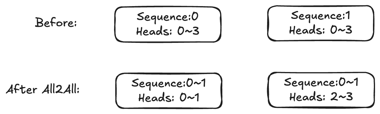
The idea: instead of moving KV during attention, rearrange the data once before attention so each rank ends up with the full sequence but only a subset of heads. Then run a vanilla local attention. Reverse the rearrangement after.
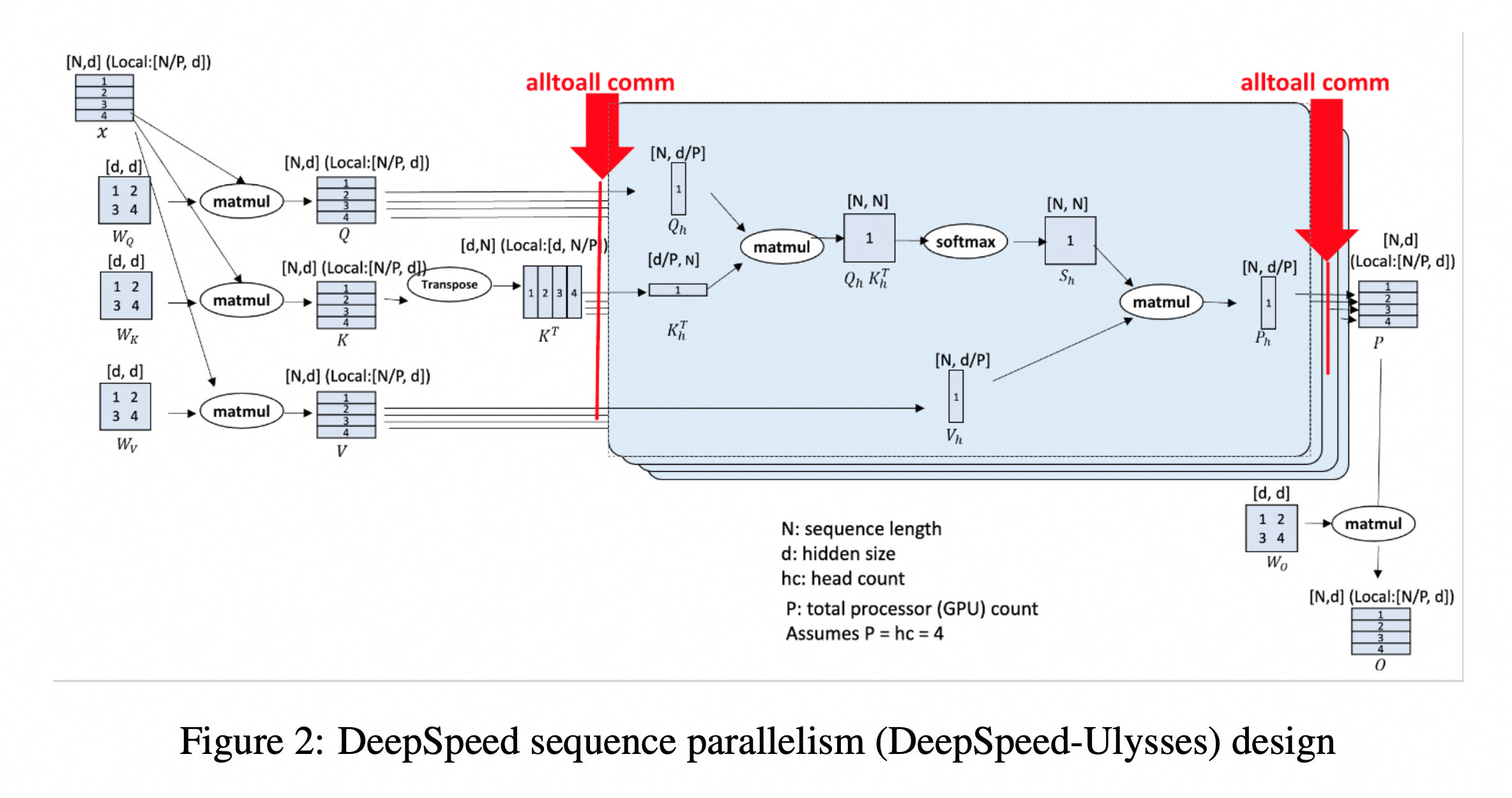
This picture shows clearly how Ulysses works, the most important thing is to understand these two alltoall communications. Without loss of generality, we explain the first alltoall communication, that turns local [N/P, d] tensor to local [N, d/P], since the last alltoall communication is symmetric.
To be short, it is split into P of [N/P, d/P] on each GPU, and then send to the corresponding GPU to get [N, d/P].
Initially GPU p holds $X^{(p)}$, one block of rows.
$$X^{(p)} \in \mathbb{R}^{\frac{N}{P} \times d}, \quad X = \begin{bmatrix} X^{(0)} \\ X^{(1)} \\ \vdots \\ X^{(P-1)} \end{bmatrix} \in \mathbb{R}^{N \times d}$$Then each local tensor $X^{(p)}$ is further split into P column-blocks:
$$X^{(p)} = \left[ X^{(p)}_{0}\;\; X^{(p)}_{1}\;\; \cdots \;\; X^{(p)}_{P-1} \right]; \quad X^{(p)}_{q} \in \mathbb{R}^{\frac{N}{P} \times \frac{d}{P}}$$During all-to-all, GPU p sends $X^{(p)}_{q}$ to GPU q and GPU q receives $X^{(0)}_{q}, X^{(1)}_{q}, \dots, X^{(P-1)}_{q}$. Then GPU q concatenates these along the sequence dimension:
$$\widetilde{X}^{(q)} = \begin{bmatrix} X^{(0)}_{q} \\ X^{(1)}_{q} \\ \vdots \\ X^{(P-1)}_{q} \end{bmatrix} \in \mathbb{R}^{N \times \frac{d}{P}}$$Mode 2: Ring (p2p) — pass the KV around
Before Step in, let's have a fast recap of the online softmax in flash attn
Keep each block's running max
m, denominatorl, and outputout; when two blocks merge, both get rescaled to the new max before being added — the code below is exactly that.
m_new = max(m_old, m_current)
l_new = exp(m_old - m_new) * l_old + exp(m_current - m_new) * l_current
out_new = (exp(m_old - m_new) * l_old * out_old + exp(m_current - m_new) * l_current * out_current) / l_new
This tells us that softmax can be computed block by block (in flash attention), and ring attn is doing the same thing, but in a $S/CP$ way.
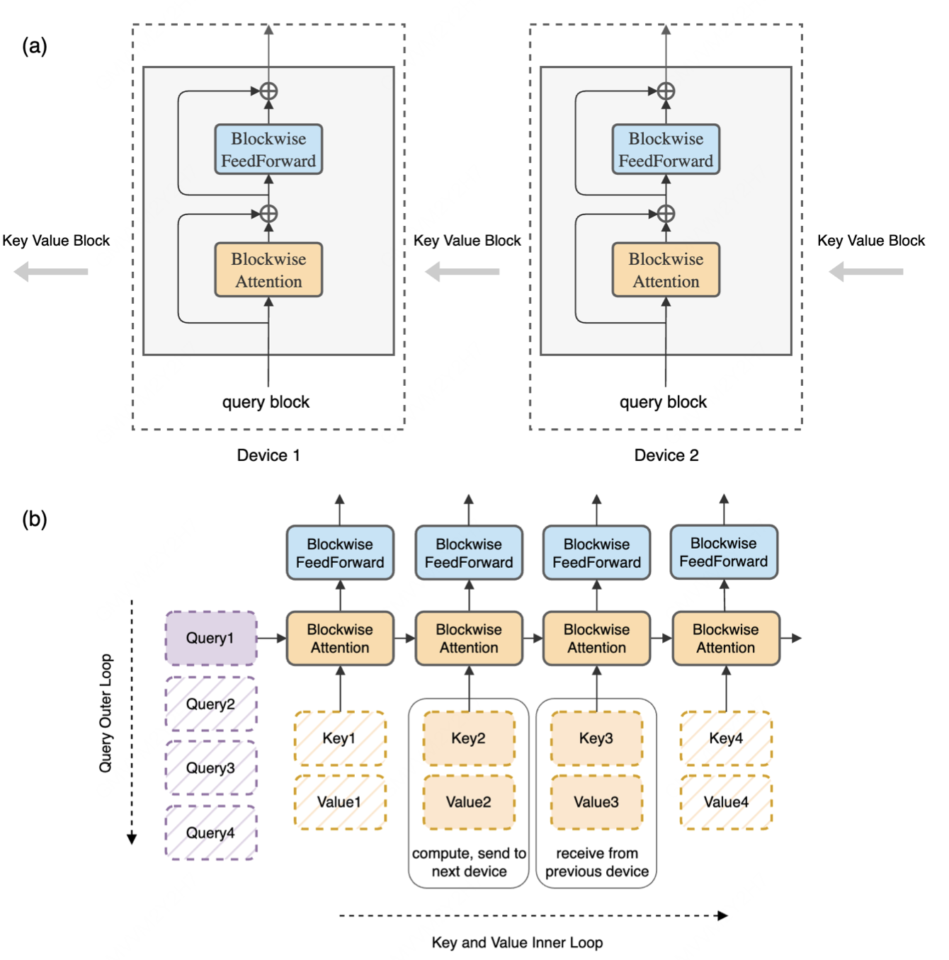
The figure is quite intuitive, since ffn is token-wise, so we only need to consider attn. At a high level, the pattern is:
- each GPU starts with its own local KV block,
- it computes attention between its local queries and the KV block currently in hand,
- meanwhile, it sends that KV block to the next GPU and receives another KV block from the previous GPU,
- it repeats this process round by round until it has seen all KV blocks it needs.
So Ring Attention turns the global attention problem into a streaming computation: compute on one KV block, pass it on, receive the next one, and keep accumulating.
The communication pattern
Each round, every GPU does exactly two communication operations: • isend its current KV package to the right neighbor • irecv the next KV package from the left neighbor
These operations are non-blocking. That means they are only launched first; the GPU does not stop and wait immediately. The actual transfer proceeds on a communication stream, while the main compute stream can continue running the attention kernel on the KV block that is already available.
This is the whole point: communication and computation can overlap.
Round    Compute (default)   | Transfer (cp_stream)
0        KV-own (buffer 0)   | send own; recv KV-A -> buffer 1
1        KV-A   (buffer 1)   | send A;   recv KV-B -> buffer 0
2        KV-B   (buffer 0)   | send B;   recv KV-C -> buffer 1
3        KV-C   (buffer 1)   | no further transfer

Send right; receive from the left.
Reuse a buffer only after its compute and transfer finish.
Compute is still flash-attn.
  Full attention (S × S)
    ├── Ring splits it into CP² blocks, each (S/CP × S/CP)     ← across GPUs
    │     └── Flash Attention splits each block into tiny tiles  ← within one GPU's SRAM
    │           └── each tile: ~128 × 128, fits in SRAM
    │
    └── Online softmax merges at BOTH levels
          - inner: tile-to-tile within Flash Attention
          - outer: chunk-to-chunk across ring steps
          - same (m, l, out) formula both times
For causal we have the zigzag assignment, to ensure the load balance.
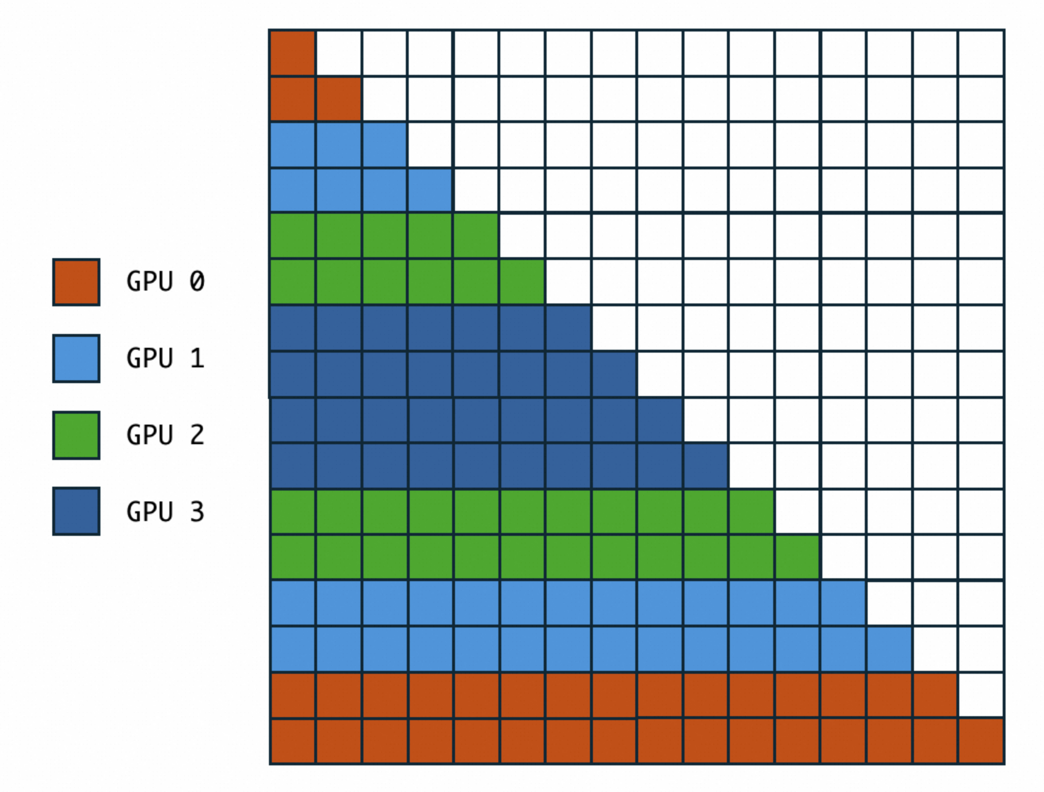
Mode 3: AllGather — just bring all KV to everyone
AllGather CP is the brute-force mode. Dead simple.
The idea: before attention, every GPU just gathers the full K and V from all CP ranks. Now every GPU has full KV in memory. Then each GPU runs plain, standard
attention — its local Q (S/CP queries) against the full K, V (all S keys/values). No ring, no partial merges, no online softmax juggling. Just normal attention
after one big collective.
Not recommended, since it is not efficient.
Hybrid CP (Hierarchical Context Parallel)
Hybrid CP splits one CP group into two nested communication levels.
Suppose you set CP=16 and cp-comm-type=a2a+p2p. Megatron then has to decide:
- which ranks should do all-to-all locally
- which groups should talk through the outer ring
That is exactly what --hierarchical-context-parallel-sizes specifies. You pass two integers [inner, outer] such that:
Example: 2 nodes x 8 GPUs = 16-way CP
Use [8, 2]:
Within each node: 8-rank a2a over NVLink.

Node 0: [R0  R1  R2  R3  R4  R5  R6  R7 ]
          |   |   |   |   |   |   |   |
Node 1: [R8  R9  R10 R11 R12 R13 R14 R15]

Each vertical link is a 2-rank p2p group over IB:
{R0,R8}, {R1,R9}, ..., {R7,R15}
inner = 8: the 8 GPUs inside each node do Ulysses-style all-to-all over NVLink.outer = 2: the two nodes communicate with each other through a ring over InfiniBand.
Why this layout works:
- all-to-all is bandwidth-heavy, so it should stay on the fast intra-node fabric
- ring is more latency-tolerant because its communication can overlap with compute
Why [2, 8] is a bad idea:
- each 2-GPU pair would do tiny all-to-alls
- the outer ring would span 8 groups across nodes
- you would push much more traffic onto InfiniBand and waste NVLink bandwidth
Mental shortcut:
inner_size= GPUs per node, or more generally GPUs inside one fast-link domainouter_size= number of such domains participating in the CP group
One constraint: in Transformer Engine v2.18's a2a path, inner_size must divide the local Q and KV head counts after TP, not just the model's total num_attention_heads, because Ulysses splits by heads**.
Dynamic CP for variable-length packing (--hybrid-context-parallel)
Despite the name, this has nothing to do with hierarchical a2a+p2p. It solves a different problem: when training with packed sequences (multiple variable-length samples concatenated into one batch), not every sub-sample needs the same CP degree. A 128K sub-sample needs many CP ranks; a 2K sub-sample fits on one GPU and gains nothing from splitting.
--max-seqlen-per-dp-cp-rank tells the scheduler the memory capacity of a single GPU, measured in tokens: "one GPU can hold at most this many tokens without OOM." The scheduler then decides, for each sub-sample, how many CP ranks to spread it across:
For example, with max-seqlen-per-dp-cp-rank = 16384:
| Sub-sample length | Needs | Assigned CP ranks |
|---|---|---|
| 8K | 8K < 16K, fits on 1 GPU | 1 |
| 32K | 32K / 16K = 2 | 2 |
| 100K | 100K / 16K = 6.25, round up to the next power of 2 | 8 |
Long samples get spread across many ranks, short samples stay local, and no GPU wastes memory on a tiny sample split across an unnecessarily large CP group.
DP is computed, not set directly.
| Parameter | Default | What it does |
|---|---|---|
--use-distributed-optimizer |
False |
Shard optimizer states across the DP group (ZeRO-1 style) |
--use-megatron-fsdp |
False |
Use Megatron's Fully Sharded Data Parallel (mutually exclusive with --use-torch-fsdp2) |
--use-torch-fsdp2 |
False |
Use PyTorch's FSDP2 implementation. Not compatible with PP, EP, MCore distributed optimizer, or fp16 |
--data-parallel-sharding-strategy |
'optim_grads_params' |
FSDP sharding mode: 'no_shard', 'optim', 'optim_grads', 'optim_grads_params' (full ZeRO-3) |
--outer-dp-sharding-strategy |
'no_shard' |
HSDP outer-group sharding: 'no_shard' (replicate) or 'optim'. Only used when Hybrid FSDP is enabled |
--num-distributed-optimizer-instances |
1 |
Number of distributed-optimizer replicas across DP (Hybrid Sharded Data Parallel degree) |
--data-parallel-random-init |
False |
Use a different random init across DP ranks |
--overlap-grad-reduce |
False |
Overlap DDP gradient reduce-scatter / all-reduce with the backward pass |
--overlap-param-gather |
False |
Overlap parameter all-gather with the forward pass (requires distributed optimizer) |
--overlap-param-gather-with-optimizer-step |
False |
Overlap the first bucket's param all-gather with the optimizer step |
--no-align-grad-reduce |
align is on by default | Let each PP stage launch grad reduces independently instead of all stages firing simultaneously |
--no-align-param-gather |
alignment on with interleaved PP; otherwise disabled | Let each PP stage launch param all-gathers independently§ |
--create-all-gather-group |
False |
Create a separate process group for all-gather to overlap reduce-scatter and all-gather |
In DP, each replica holds a full copy of its model partition (or, with sharding, a complete logical replica of that partition). It's also the only axis you don't set directly — DP falls out of the math:
$$\text{DP} = \frac{\text{world\_size}}{TP \times PP \times CP}$$You decide TP, PP, CP for the dense view (and EP, expert_TP for the expert view); DP and expert_DP are the leftovers. The "Relation between Parallelism" section below works through how the same world_size factors into both views simultaneously.
The whole DP story is then about what happens to that full copy: keep it whole (DDP), shard it (ZeRO/FSDP), or partially shard it (HSDP). Each algorithm is a different point on the memory-vs-communication trade curve.
For a simplified 7B example with bf16 params/grads and fp32 Adam moments, excluding fp32 master parameters, each DP rank holds:
| Tensor | Size in bf16 (params) | Size in fp32 (Adam) |
|---|---|---|
| Parameters | 14 GB | — |
| Gradients | 14 GB | — |
| Optimizer momentum | — | 28 GB |
| Optimizer variance | — | 28 GB |
| Total per rank | ~84 GB |
That's already over an 80 GB H100 — and 7B is small. With DP=8, every replica wastes 7× the memory it needs to. The DP algorithms below are progressively more aggressive ways to share that wasted memory across the DP group.
Default behavior. No DP flags set.
The baseline. Every DP rank holds the full state. After backward:
Backward done on every rank → each rank has its local 14 GB grad tensor
                            → AllReduce across DP group  (1 collective)
                            → every rank now has the same averaged grad
                            → optimizer step runs locally on every rank (redundantly)
Comm: 1 AllReduce per step (just gradients). Memory: nothing saved. Every rank holds full params + grads + optimizer state.
This is what you get if you set none of the DP flags. It's the simplest, but the most memory-hungry.
Enabled by
--use-distributed-optimizer. Megatron's own implementation, conceptually identical to DeepSpeed's ZeRO-1.
The cheapest, biggest memory win. Optimizer state is the largest single component (Adam keeps two fp32 tensors per parameter — momentum and variance, ~56 GB for our 7B model). Sharding it across DP ranks recovers most of the wasted memory immediately.
Each rank now holds:
  - Full params      (still 14 GB)
  - Full grads       (still 14 GB)
  - 1/DP optim state (e.g., 7 GB instead of 56 GB at DP=8)
The communication pattern flips:
Backward → ReduceScatter grads (instead of AllReduce)
           Each rank now holds 1/DP of the grad — the slice corresponding to
           its 1/DP of the optimizer state.

Optimizer → Local optimizer step on the 1/DP slice.

Forward (next step) → AllGather params, because each rank only updated its slice.
Comm: 1 ReduceScatter (grads) + 1 AllGather (params) per step. Same total volume as DDP's AllReduce, just split into two halves.
Memory: optimizer state shrinks by DP×. For our 7B example, recovers ~50 GB per rank.
This is the highest-leverage move you can make. Almost every production training job uses at least this.
Enabled by
--use-megatron-fsdp(which requires--use-distributed-optimizer). The depth is controlled by--data-parallel-sharding-strategy, which defaults to'optim_grads_params'(full ZeRO-3) when FSDP is enabled.
Going further. The --data-parallel-sharding-strategy flag exposes four levels of sharding aggressiveness:
| Strategy | What it shards | Conceptually |
|---|---|---|
'no_shard' |
Nothing | DDP |
'optim' |
Optimizer state | ZeRO-1 |
'optim_grads' |
Optimizer + gradients | ZeRO-2 |
'optim_grads_params' |
Optimizer + grads + parameters | ZeRO-3 / Full FSDP |
The 'optim' and 'optim_grads' strategies save more memory at modest extra comm cost. Going to full ZeRO-3 introduces a qualitatively new behavior worth understanding.
The runtime cost of sharding parameters. With ZeRO-3, each GPU only holds 1/DP of every layer's parameters. But to actually run a layer's forward, you need the whole weight matrix for that layer. So Megatron-FSDP issues a just-in-time AllGather before each layer's forward, materializes the full weight for one matmul, then releases it:
Layer 1 forward:  AllGather params  →  matmul  →  release
Layer 2 forward:  AllGather params  →  matmul  →  release
...
One AllGather per layer per forward. Same on backward. This is much more comm volume than ZeRO-1, but the reward is that the param memory itself is sharded — the biggest possible memory saving.
Megatron-FSDP enforces a hard requirement: it only works when --use-distributed-optimizer is also set. The two flags must travel together.
For the full-shard setup below, use
--use-megatron-fsdpwith'optim_grads_params'and--num-distributed-optimizer-instances > 1. Companion flag--outer-dp-sharding-strategycontrols outer-group behavior.
Full ZeRO-3 has a problem at large scale. When DP is large enough to cross node boundaries, the per-layer AllGather goes over InfiniBand (~50 GB/s) instead of NVLink (~600 GB/s). At 60 layers × 1 forward + 1 backward, you pay 120 cross-node AllGathers per micro-batch. The comm dominates wall-clock.
HSDP fixes this by splitting the DP dimension into two nested levels:
HSDP layout (DP=64, num_instances=8):

  Inner level (within each node, 8 GPUs):    Full ZeRO-3 sharding
  Outer level (across the 8 nodes):          Replication

  Node 0           Node 1           ...    Node 7
  +-------------+  +-------------+         +-------------+
  | GPU 0: 1/8  |  | GPU 0: 1/8  |         | GPU 0: 1/8  |
  | GPU 1: 1/8  |  | GPU 1: 1/8  |   ...   | GPU 1: 1/8  |
  | ...         |  | ...         |         | ...         |
  | GPU 7: 1/8  |  | GPU 7: 1/8  |         | GPU 7: 1/8  |
  |             |  |             |         |             |
  | Full copy   |  | Full copy   |         | Full copy   |
  | of model    |  | of model    |         | of model    |
  +-------------+  +-------------+         +-------------+
         ^                ^                       ^
     replicas of each other (the "outer" axis = 8 replicas)
What changes:
- The per-layer AllGather (params) → only across the inner group of 8 GPUs → NVLink only, fast
- The gradient sync (once per step) → across the outer group of 8 nodes → cross-node IB, but it had to happen anyway in any DP scheme
- Memory cost: each node now holds a full copy of the model. So HSDP uses
outer×more memory than full ZeRO-3 — in the diagram, 8 replicas instead of 1. Worth it because cross-node param AllGathers are gone.
The companion --outer-dp-sharding-strategy controls the outer group:
'no_shard'(default): outer is pure replication — the picture above'optim': outer also shards optimizer state across replicas. Saves more memory, costs more cross-node comm. Only valid when inner is'optim_grads_params'.
In Megatron, set --num-distributed-optimizer-instances=N where N is the desired outer degree (number of replicas). Inner = DP / N.
Enabled by
--use-torch-fsdp2. Mutually exclusive with--use-megatron-fsdp.
Megatron also exposes PyTorch's native FSDP2 as an alternative implementation of the same ZeRO-3 algorithm. It's largely experimental — the upstream code lists six incompatibilities:
- Not compatible with PP (pipeline parallelism)
- Not compatible with EP (expert parallelism)
- Not compatible with MCore distributed optimizer
- Not compatible with fp16
- Not compatible with gradient accumulation fusion
- Requires
--ckpt-format torch_distortorch_dcp, plus--untie-embeddings-and-output-weights
For production large-scale training (which usually involves PP and/or EP), FSDP2 isn't a realistic choice. It exists for small experiments and for users committed to the PyTorch-native stack.
One ZeRO-2-like toggle worth noting: --torch-fsdp2-no-reshard-after-forward keeps full params in memory between forward and backward, avoiding the backward AllGather. Parameters are still resharded after backward by default; this flag alone does not keep them permanently replicated††.
The same overlap recipe we've seen for PP, CP, and EP applies to DP. ZeRO's ReduceScatter and AllGather are in the critical path; both can be hidden:
| Flag | What it hides |
|---|---|
--overlap-grad-reduce |
Hides ReduceScatter behind backward compute |
--overlap-param-gather |
Hides AllGather behind forward compute (requires distributed optimizer) |
--overlap-param-gather-with-optimizer-step |
Starts the first param-bucket's AllGather while optimizer step on later buckets is still running. Requires interleaved PP. |
Two PP×DP interaction flags:
--no-align-grad-reduce— disable the synchronized launch of grad reduces across PP stages (alignment defaults ON)--no-align-param-gather— same, for param gathers (alignment defaults ON with interleaved PP; otherwise disabled)§
When alignment is on, the pipeline schedule aligns the launch points of DP collectives, rather than enforcing an exact wall-clock instant§. Predictable, but can over-subscribe NCCL. Disabling alignment lets each PP stage fire when it's actually ready — better concurrency, more complex scheduling.
One more optimization: --create-all-gather-group creates a separate process group for AllGather so it can run concurrently with ReduceScatter (instead of sharing one group's resources).
Let $P$, $G$, $O$ be a model partition's parameter, gradient, and optimizer-state bytes, and $d$ the sharding-group size (in the CP=1 examples here, $d = DP$; for HSDP with $N$ replicas, let $h = d/N$ be the inner-group size).
| Algorithm | Per-rank memory | Comm volume per step | Best for |
|---|---|---|---|
| DDP | $P+G+O$ | 1 AllReduce (grads) | Small models that fit |
ZeRO-1 (--use-distributed-optimizer) |
$P+G+O/d$ | 1 RS + 1 AG | Default for most training |
ZeRO-2 ('optim_grads') |
$P+(G+O)/d$ | 1 RS + 1 AG | Mid-range memory pressure |
ZeRO-3 / Full FSDP ('optim_grads_params') |
$(P+G+O)/d$ | Per-layer AG + per-step RS | Maximum memory savings, DP within fast-link domain |
HSDP (--num-distributed-optimizer-instances=N, outer 'no_shard') |
$(P+G+O)/h$ | Per-layer AG/RS intra-node + per-step AllReduce cross-node‡‡ | Large DP that crosses nodes |
For the 7B example above ($P=14$, $G=14$, $O=56$ GB) at $d=8$, ZeRO-1/2/3 give 35 / 22.75 / 10.5 GB — 41.7% / 27.1% / 12.5% of the 84 GB baseline; HSDP's fraction is $1/h$ (12.5% at $h=8$), not a fixed 50%. These are idealized model-state formulas, not peak-memory guarantees.
Decision tree:
- Model fits in DDP memory? → leave everything off. You get DDP.
- Need more memory? →
--use-distributed-optimizer(ZeRO-1). Recovers most of the optimizer state. Almost always worth it.- Still not enough? → add
--use-megatron-fsdpand pick'optim_grads'or'optim_grads_params'via--data-parallel-sharding-strategy.- Full ZeRO-3 with DP crossing nodes? → add
--num-distributed-optimizer-instances=Nto switch to HSDP. Inner = DP / N.
expert_DPis computed separately because the expert view ofworld_sizefactors differently: $\text{expert\_DP} = \text{world\_size} / (\text{expert\_TP} \times PP \times EP)$. The same DP/HSDP/FSDP machinery applies to expert parameters within their own DP group. The "Relation between Parallelism" section below works through how the dense and expert views coexist on the same physical GPUs.
So far we've treated TP, PP, CP, EP, SP, and DP one at a time. But in a real job, all of them coexist on the same GPUs. This section answers: how do they fit together, and how does a single global rank know which group it belongs to in each dimension?
The short answer: upstream Megatron-LM uses two separate "rank grids" — one for dense/attention parameters, one for MoE expert parameters. Each grid is a 4D factorization of world_size. A single GPU sits in both grids simultaneously, with different coordinates in each.
Out of the six things, you only directly set four (or five, if you override expert_TP):
| Quantity | How it's set |
|---|---|
TP |
--tensor-model-parallel-size |
PP |
--pipeline-model-parallel-size |
CP |
--context-parallel-size |
EP |
--expert-model-parallel-size |
expert_TP |
--expert-tensor-parallel-size (defaults to TP if not set) |
SP |
--sequence-parallel (a flag, not a size — auto-disabled if TP=1) |
DP |
computed: world_size / (TP × PP × CP) |
expert_DP |
computed: world_size / (expert_TP × EP × PP) |
So world_size decomposes into:
Two products, both equal to world_size. SP isn't in either product because SP doesn't create a process group — it just reuses the TP group (see SP section).
Megatron has two separate worlds:
- Dense world: TP × PP × CP × DP — for attention, dense FFN, embeddings
- Expert world: expert_TP × PP × EP × expert_DP — for MoE expert FFNs
The single most important thing to grasp: the same set of physical GPUs is partitioned two different ways, depending on which weights you're looking at.
The upstream code (megatron/core/parallel_state.py) makes this explicit by constructing two RankGenerator objects:
# View #1 — for attention / dense layers
decoder_rank_generator = RankGenerator(
    tp = tensor_model_parallel_size,
    ep = 1,                          # ← EP forced to 1
    dp = data_parallel_size,
    pp = pipeline_model_parallel_size,
    cp = context_parallel_size,
)

# View #2 — for MoE expert layers
expert_decoder_rank_generator = RankGenerator(
    tp = expert_tensor_parallel_size,
    ep = expert_model_parallel_size,
    dp = expert_data_parallel_size,  # = world_size / (eTP × EP × PP)
    pp = pipeline_model_parallel_size,
    cp = 1,                          # ← CP forced to 1
)
Side by side:
tp |
ep |
dp |
pp |
cp |
|
|---|---|---|---|---|---|
| View #1 (dense) | TP | 1 | DP | PP | CP |
| View #2 (expert) | eTP | EP | eDP | PP | 1 |
Hard rule from the code (
RankGenerator.__init__, line ~452):assert ep == 1 or cp == 1EP and CP cannot both be greater than 1 in the same grid here. This is a restriction of Megatron's
RankGeneratorimplementation. This is why upstream uses two separate generators.
The reason is how the two grids account for sequence partitioning and replication:
Attention weights (View #1): Each CP rank still owns its own copy of Q/K/V/O matrices to compute attention on its sequence chunk. CP splits the sequence, not these weights. With more CP at fixed world size, fewer independent data replicas fit, so DP shrinks.
Expert weights (View #2): Each rank runs its local experts on the tokens dispatched to it. The experts don't care which sequence chunk those tokens came from. So CP doesn't need a separate coordinate in the expert grid; these ranks are accounted for by expert_DP, alongside the other replication factors.
Concrete numbers for a 64-GPU job with TP=4, PP=2, CP=8, EP=4, expert_TP=1:
tp |
ep |
dp |
pp |
cp |
Product | |
|---|---|---|---|---|---|---|
| View #1 | 4 | 1 | 1 | 2 | 8 | 4×1×1×2×8 = 64 ✓ |
| View #2 | 1 | 4 | 8 | 2 | 1 | 1×4×8×2×1 = 64 ✓ |
DP = 1 means one independent data replica for the dense view — but not a single copy of the attention weights: as noted above, each CP rank still holds its own Q/K/V/O copy, so before any sharding the weight partition exists in CP × DP = 8 copies. expert_DP = 8 means 8 replicas for experts. The CP factor "moved" from the sequence axis to the replication side.
Once the dimensions are fixed, the system needs to decide which physical GPU gets which (tp, pp, cp, dp) tuple. That's controlled by the order parameter of RankGenerator:
order = "tp-cp-ep-dp-pp"(default): TP varies fastest, PP slowest.order = "tp-cp-ep-pp-dp": PP varies before DP (HSDP-friendly).
"Varies fastest" means: consecutive global_rank IDs differ in that dimension first. Since consecutive global_ranks usually land on adjacent physical GPUs (same node, NVLink), the fastest-varying dimension gets the fastest interconnect.
Concrete: 8 GPUs with TP=2, CP=2, DP=2, PP=1, default order:
global_rank → (tp, cp, dp, pp)
   0        →  (0, 0, 0, 0)
   1        →  (1, 0, 0, 0)   ← TP varies first
   2        →  (0, 1, 0, 0)
   3        →  (1, 1, 0, 0)
   4        →  (0, 0, 1, 0)
   5        →  (1, 0, 1, 0)
   6        →  (0, 1, 1, 0)
   7        →  (1, 1, 1, 0)

TP groups (vary tp, fix others): {0,1}, {2,3}, {4,5}, {6,7}   ← intra-node
CP groups (vary cp, fix others): {0,2}, {1,3}, {4,6}, {5,7}
DP groups (vary dp, fix others): {0,4}, {1,5}, {2,6}, {3,7}   ← may cross nodes
This is why the order matters: TP traffic is the heaviest (one collective per matmul block), so TP groups must land on the fastest links. DP traffic is the lightest (one gradient sync per optimizer step), so DP groups can stretch across nodes. PP traffic is sparse activation hand-offs, so it can also stretch across nodes (typically placed last).
Most of the time, the dense and expert views are independent — you change one without affecting the other. But there is one constraint the upstream code enforces (parallel_state.py line ~803):
assert (
    order.endswith("pp")
    or pipeline_model_parallel_size == 1
    or expert_data_parallel_size == data_parallel_size
), "When not using pp-last rank ordering, the data parallel size of the attention and moe layers must be the same"
In words: if PP > 1 and the rank order does not put pp last, then expert_DP must equal DP. Otherwise the dense and expert views would form different pipeline groups, breaking the shared pipeline layout.
This is the one place where the two factorizations are not fully independent. In practice, most jobs use the default order ending in pp, so this constraint rarely fires.
Putting it together, every physical GPU in a Megatron-LM job carries two coordinate tuples simultaneously:
GPU (global_rank = R)
  ├── In View #1 (dense): (tp_rank, pp_rank, cp_rank, dp_rank)
  │   └── Belongs to: TP group, PP group, CP group, DP group
  │       Used when forward/backward hits attention or dense FFN
  │
  └── In View #2 (expert): (etp_rank, pp_rank, ep_rank, edp_rank)
      └── Belongs to: expert_TP group, PP group (same as above), EP group, expert_DP group
          Used when forward/backward hits MoE FFN
The two views share pp_rank (same layer-stack split), but everything else is independent. When the model's forward pass enters an attention layer, it calls collectives on View #1's groups. When it enters an MoE FFN, it calls collectives on View #2's groups. Same GPU, different process groups, called from different layers.
Mental model:
world_sizeis fixed by your job submission.- You decide how to factor it for dense weights → that picks
TP,PP,CP, leavingDPas the leftover.- You decide how to factor it for expert weights → that picks
expert_TP,EP(PP is shared), leavingexpert_DPas the leftover.- The
orderstring decides which physical GPUs get which coordinates.RankGenerator.get_ranks(token)walks the grid and returns each set of ranks that should form one process group.- Every collective call in the model targets one of these pre-built groups.
That's the whole machine. Six knobs (TP/PP/CP/EP/eTP/order), two derived quantities (DP/eDP), one assertion to keep them consistent — and from that, every NCCL group in the job is constructed.
- 1
https://docs.nvidia.com/nemo/megatron-bridge/latest/parallelisms.html NeMo Megatron Bridge: parallelisms overview (maps concepts to training flags). ↩
- 2
https://arxiv.org/abs/2104.04473 Megatron-LM: efficient large-scale training on GPU clusters (tensor + pipeline parallelism, schedules, MoE integration as used in the codebase lineage). ↩
- 3
https://arxiv.org/abs/1909.08053 Megatron-LM: training multi-billion-parameter models with model (tensor) parallelism. ↩
- 4
https://arxiv.org/abs/1811.06965 GPipe: pipeline parallelism with micro-batching (bubble vs. memory tradeoff baseline many Megatron-style schedules build on). ↩
- 5
https://arxiv.org/abs/2205.05198 Reducing activation recomputation in large transformers (Megatron-style sequence parallelism paired with tensor parallel groups). ↩
- 6
https://arxiv.org/abs/2309.14509 DeepSpeed-Ulysses: extreme long-sequence training via head-dimension partitioning (all-to-all “Ulysses” pattern echoed in CP-a2a style paths). ↩
- 7
https://arxiv.org/abs/2101.03961 Switch Transformers: scaling to trillion-parameter models with expert routing (MoE / expert-parallel motivation). ↩
- 8
https://lilianweng.github.io/posts/2021-09-25-train-large/#training-parallelism How to Train Really Large Models on Many GPUs?
- §
Megatron Core
core_v0.19.2, commit4b4acac9a1d28ea6829c8d4f566d75698a21249d: pipeline schedules (VPP warmup and collective launch alignment), argument validation (parameter-gather alignment), and TransformerConfig (EP-overlap requirements). ↩ - **
Transformer Engine
v2.18, context_parallel.py: the a2a attention path checks local Q/KV head divisibility by the a2a group size. ↩ - ††
PyTorch
v2.9.0, fully_shard and FSDPModule:reshard_after_forward=Falseretains unsharded parameters into backward; resharding after backward is controlled separately. ↩ - ‡‡
Megatron Core
core_v0.19.2, Megatron-FSDP guide: HSDP shards within the inner group and all-reduces gradients across outer replicas before the optimizer step. ↩
Broadcast
One source rank owns a tensor, and after Broadcast every rank gets the same tensor.
If rank 0 owns $x$, then after Broadcast, every rank owns the same $x$.
Reduce
This combines values across ranks and places the reduced result on one destination rank.
For summation,
$$y = \sum_{r=0}^{N-1} x^{(r)}$$and after Reduce, only the destination rank owns $y$.
AllReduce
Every GPU gets the full reduced result:
$$y = \sum_{r=0}^{N-1} x^{(r)}$$and after AllReduce, every rank owns the whole y.
Scatter
One source rank starts with the full tensor split into chunks and sends one chunk to each rank.
If
$$y = [y_0, y_1, \dots, y_{N-1}]$$then after Scatter, rank $i$ gets $y_i$
ReduceScatter
This does two things at once: 1. Reduce across ranks 2. Scatter the result into chunks
If y is split into N chunks,
$$y = [y_0, y_1, \dots, y_{N-1}]$$then after ReduceScatter, rank i gets only chunk y_i.
So each rank gets:
$$y_i = \left(\sum_{r=0}^{N-1} x^{(r)}\right)_i$$That means: correct reduced result, but only one slice of it.
Gather
This is the opposite of Scatter: each rank starts with one chunk, and one destination rank collects all chunks into the full tensor.
If rank $i$ owns $y_i$
then after Gather, the destination rank owns
$$y = [y_0, y_1, \dots, y_{N-1}]$$AllGather
This is the opposite pattern: each rank starts with one chunk, and everyone exchanges chunks so that every rank gets the full tensor.
If rank i starts with y_i, then after AllGather every rank gets:
$$y = [y_0, y_1, \dots, y_{N-1}]$$All-to-All
Each rank splits its local tensor into $N$ chunks and sends one chunk to every other rank, while also receiving one chunk from every other rank.
If rank $r$ starts with
$$x^{(r)} = [x^{(r)}_0, x^{(r)}_1, \dots, x^{(r)}_{N-1}]$$then after All-to-All, rank $i$ gets
$$[x^{(0)}_i, x^{(1)}_i, \dots, x^{(N-1)}_i]$$Before we get into the parallelism strategies, let's pin down the vocabulary used throughout the blog. Distributed training has a small zoo of words for "the thing running on a GPU," and confusing them makes the later sections much harder to read.
GPU (device)
A single accelerator chip. In modern training setups, a typical machine has 8 GPUs, all visible via nvidia-smi as devices cuda:0 through cuda:7.
Node One physical machine — usually one server with 8 GPUs, its own host CPU, RAM, and NICs. GPUs within a node talk to each other over fast intra-node links (NVLink / NVSwitch). GPUs in different nodes talk over the slower inter-node fabric (InfiniBand / RoCE).
Process One operating-system process running the training script. In Megatron-LM (and almost every modern framework), there is one process per GPU. The process owns its GPU, holds its slice of the model, and runs forward/backward.
So an 8-GPU node runs 8 processes in parallel. A 64-GPU job (8 nodes × 8 GPUs) runs 64 processes total. They communicate through NCCL (or Gloo) collectives, not shared memory.
Every process has two integer IDs:
local_rank
The process's index within its own node, ranging from 0 to gpus_per_node - 1. On an 8-GPU node, local ranks are 0..7. This is the ID you use to pick which GPU to bind to:
torch.cuda.set_device(local_rank)
global_rank (often just called rank)
The process's index across the entire job, ranging from 0 to world_size - 1. On a 64-GPU job, global ranks are 0..63. This is the ID NCCL uses to address messages between processes.
world_size
The total number of processes in the job. For 8 nodes × 8 GPUs, world_size = 64.
The relationship is straightforward when nodes are uniform:
global_rank = node_id * gpus_per_node + local_rank
A process group is a subset of ranks that participate in the same collective communication call (AllReduce, AllGather, etc.). Megatron-LM creates several overlapping process groups, one per parallelism dimension:
| Group | Members | What they exchange |
|---|---|---|
| TP group | The TP ranks that hold pieces of the same layer | Activations after sharded matmuls (AllReduce / ReduceScatter) |
| PP group | The PP ranks that hold consecutive layer chunks | Forward/backward activations between stages (P2P send/recv) |
| CP group | The CP ranks that hold pieces of the same sequence | KV chunks (ring) or head subsets (Ulysses) |
| EP group | The EP ranks that hold disjoint sets of MoE experts | Tokens routed to remote experts (all-to-all) |
| DP group | The DP ranks that replicate the same model partition | Gradients (AllReduce or ReduceScatter for FSDP) |
Each rank belongs to all of these groups simultaneously — its position is one coordinate in a multi-dimensional grid. For example, with TP=4, PP=2, CP=8, DP=1 on 64 GPUs, a single rank has a (tp_rank, pp_rank, cp_rank, dp_rank) tuple identifying it within each group.
Takeaway: a "rank" is an integer ID for a process, not a role. The same process is
tp_rank=2in the TP group,pp_rank=0in the PP group,cp_rank=5in the CP group, and so on — all at the same time. Process groups are the primitive that makes this possible.